FORMULAE
Spreadsheet formulae usually contain numbers, arithmetical operators and cell references. They can be typed in directly or Excel can help build them for you. You can use all the standard mathematical operators in your formula; e.g. () + – / *. A spreadsheet is an excellent platform to work out sums and functions.
ENTERING A FORMULA
Activate the cell in to which you want to enter the formula.
Enter “= (equals)”
Type in the formula by hand or:
Click in to each of the cells, adding the relevant operators (+/* – etc.) where appropriate.
Click on the tick to accept the formula or press enter.
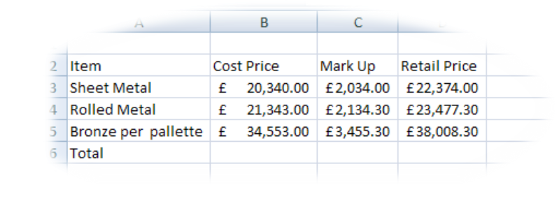
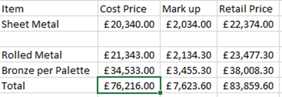
In the example below; column B holds information on the Cost Price of the products listed in column A.
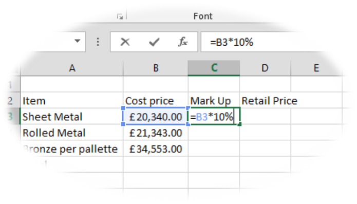
Column C requires a formula to calculate a 10% Mark Up on the Cost Price for each product. Cell D3 requires the total of the Cost Price and the Mark Up columns giving the Retail Price.
Once the Mark Up price has been calculated, working out the Retail Price is quite easy.Type = in cell D3 (this is the cell where you want the answer to appear), click in to cell B3, select the plus option and click in to cell C3.
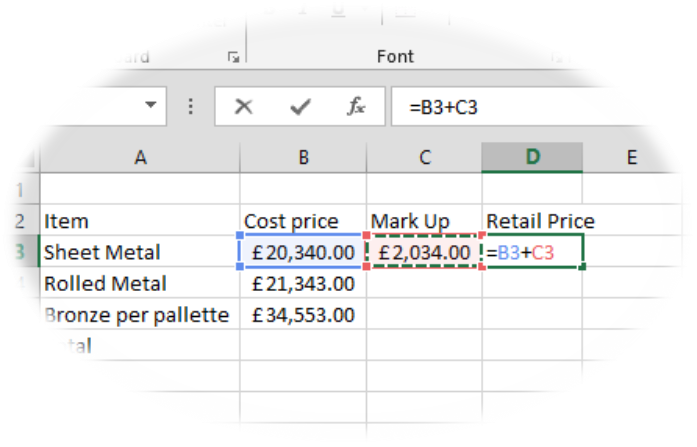
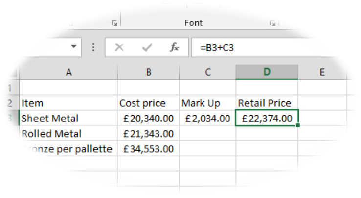
The last thing that you should always do is check the formula, if you are happy with it, click the tick or press enter.
The next step in the process is utilising the AutoFill feature to fill the formula down each row. There are always several ways to complete the task in Excel. In the previous example, the formula that you have just completed to work out the Retail Price can be repeated for each product. It is quite permissible for you to repeat the process and type each formula out manually on each row. However, because both parts of the formula are on the same row in this example you can use the AutoFill feature.
AutoFill
The small black cross will appear when you move your mouse pointer over the bottom right hand corner of any selected cell or cells.
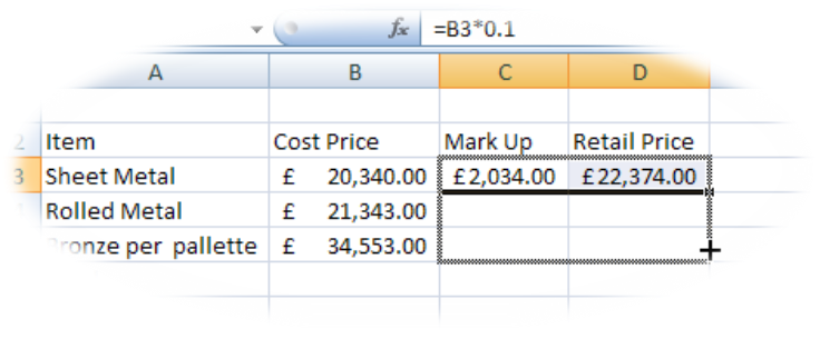
Once the small black cross appears simply click and drag down the appropriate number of rows and the formula will be copied down. Note: You can also double click the small black cross and the formula will fill down, until it hits a gap or information in a cell.
The next step in our little example is to total each column. There are two ways that we can do this. One, use the formula =B3+B4+B5 etc. or two, use a Function called AutoSum. This function has been designed to add up lists or ranges, as they are called in Excel.
Both examples will provide the correct result however; you will be restricted by using multiple + symbols.
AutoSum function
The AutoSum function is the most common function used Excel and therefore it appears in more than one place on the Ribbon. The AutoSum feature is at the right side of the home ribbon.
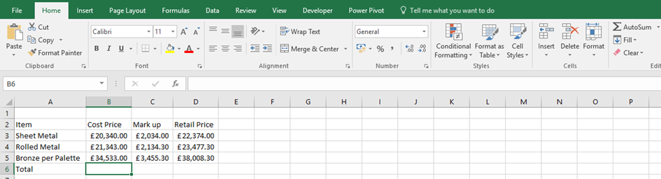
The first thing you must do is click in the cell where you want the answer to appear. Then click the AutoSum button.
The function will guess what you want to add up, you must check that it is correct before clicking the tick or pressing enter.
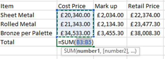
In the example below the function has guessed correctly so it is safe to click the tick or press enter.
Once again, all the elements in this formula are in the same column so you can use the AutoFill feature to drag the formula in to column D.
Make sure that you see the small black cross in the bottom right hand corner before you start to drag.
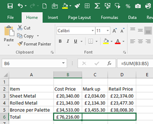
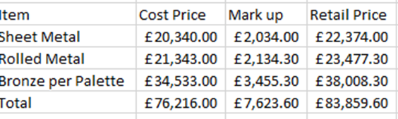
The results are displayed under each column as shown below.
In the following example, I want to look at what happens when the AutoSum or any other function for that matter does not pick up the correct range of cells.
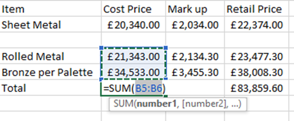
As you can see from the example above the blank row has caused a problem.
The AutoSum feature guesses that you want to add up the figures up to the gap and not beyond it.
You will now need to intervene if you want all of column B to be added together.
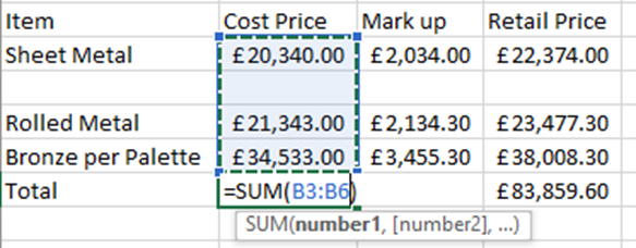
In the example above, I have selected the first cell that I want to add and then with the large white cross, selected the rest of the cells.
Make sure that you check the formula, before clicking the tick.
| Steve Says I cannot emphasise enough; how important it is to check the cell references on the formula bar. I always recommend that new users select the tick on the formula bar to accept formulae rather than pressing enter, that way they are always physically checking a formula before accepting it. If things go wrong, click the Red Cross on the Formula bar and start again. |
Sums and functions are easy to do in Excel but checking the formula is the most important part when dealing with sums and functions.
Courses
Search for courses here
Search for online courses here

